Lens JBrowse2
What is JBrowse?
JBrowse is a genome browser and platform for visualizing genomic data. It provides an interactive interface for browsing genomic features, such as genes, transcripts, and variants, as well as the ability to customize the display and add your own data tracks.
Citation: JBrowse 2: A modular genome browser with views of synteny and structural variation (2022). bioRxiv. https://doi.org/10.1101/2022.07.28.501447
Linear Genome Views
- Lens culinaris CDC Redberry v2.0 (Lcu.2RBY)
- Lens culinaris CDC Greenstar v1.0 (Lcu.1GRN)
- Lens ervoides IG 72815 v1.0 (Ler.1DRT)
- Lens lamottei IG 110813 v1.0 (Lla.1ESP)
- Lens nigricans ILWL 25 v1.0 (Lni.1VIC)
- Lens odemensis IG 72623 v1.0 (Lod.1TUR)
- Lens orientalis BGE 016880 v1.0 (Lor.1WPS)
- Lens tomentosus IG 72805 v1.0 (Lto.1BIG)
Resources
- Introduction to our Lens JBrowse2 (powerpoint download)
- Official JBrowse2 user guide
- JBrowse2 Genome Hub - database of JBrowses
Case studies:
- 1. Multi-sample variant tracks - adding your own qualitative phenotypes
- 2. Viewing your own GWAS results as a track
- 3. Demonstrating synteny between Lens species
1. Multi-sample variant tracks - adding your own qualitative phenotypes
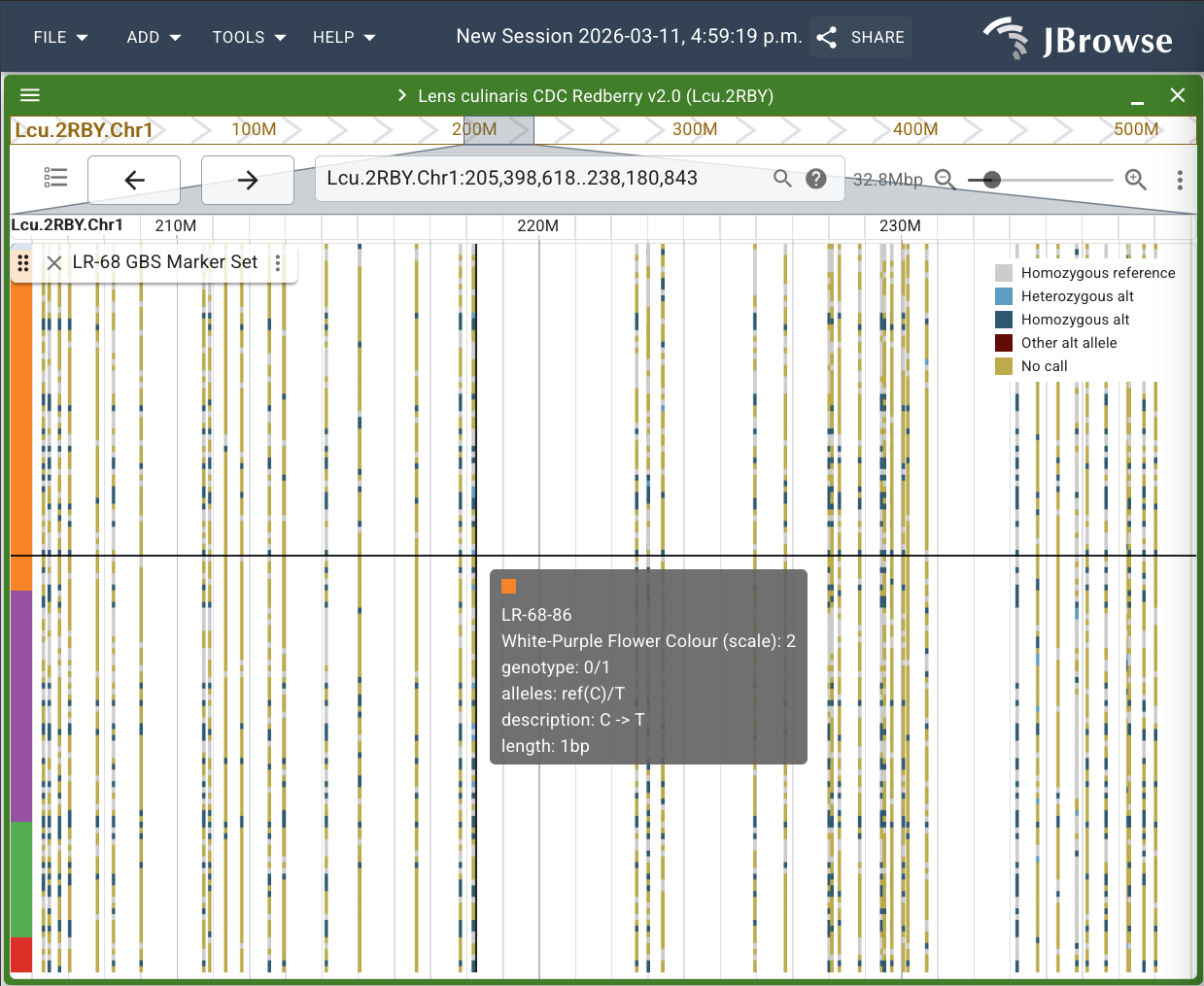
This will walk you through how to colour samples on a multi-sample variant track in JBrowse. This can be useful to group or highlight genotypes based on a particular phenotype or based on any metadata you want, such as geographic origin. For example, you could colour samples based on their resistance or susceptibility to a particular disease. This can help you identify patterns in the data.
For this example, we will colour the samples of the LR-68 GBS Marker Set on the Lcu.2RBY assembly in JBrowse based on the segregating trait white-purple flower colour. We will use a subset of data collected by Didier Socquet-Juglard for work done on this research experiment: https://knowpulse.usask.ca/experiment/EVOLVES-shattering-LR68
Download white-purple flower colour trait for LR-68
Navigate to the Lcu.2RBY assembly in JBrowse and select the LR-68 GBS Marker Set track in the track list.
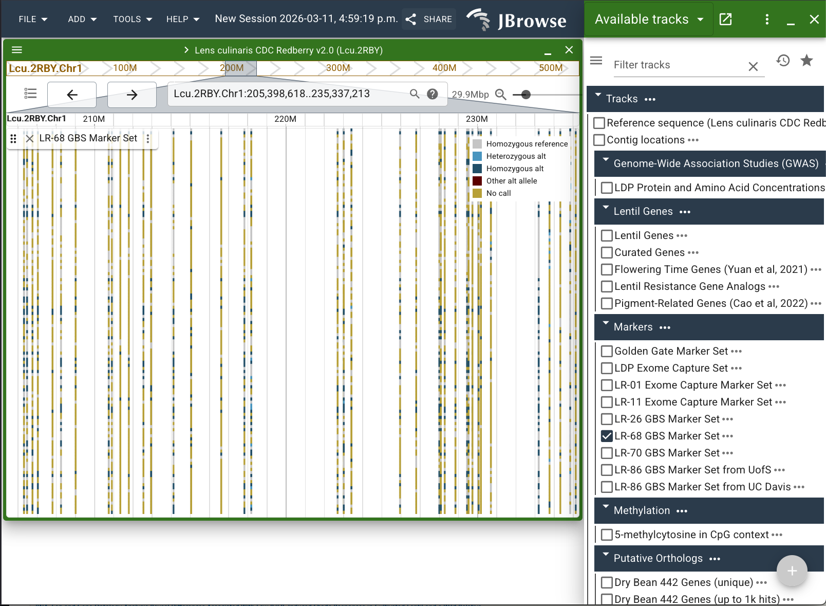
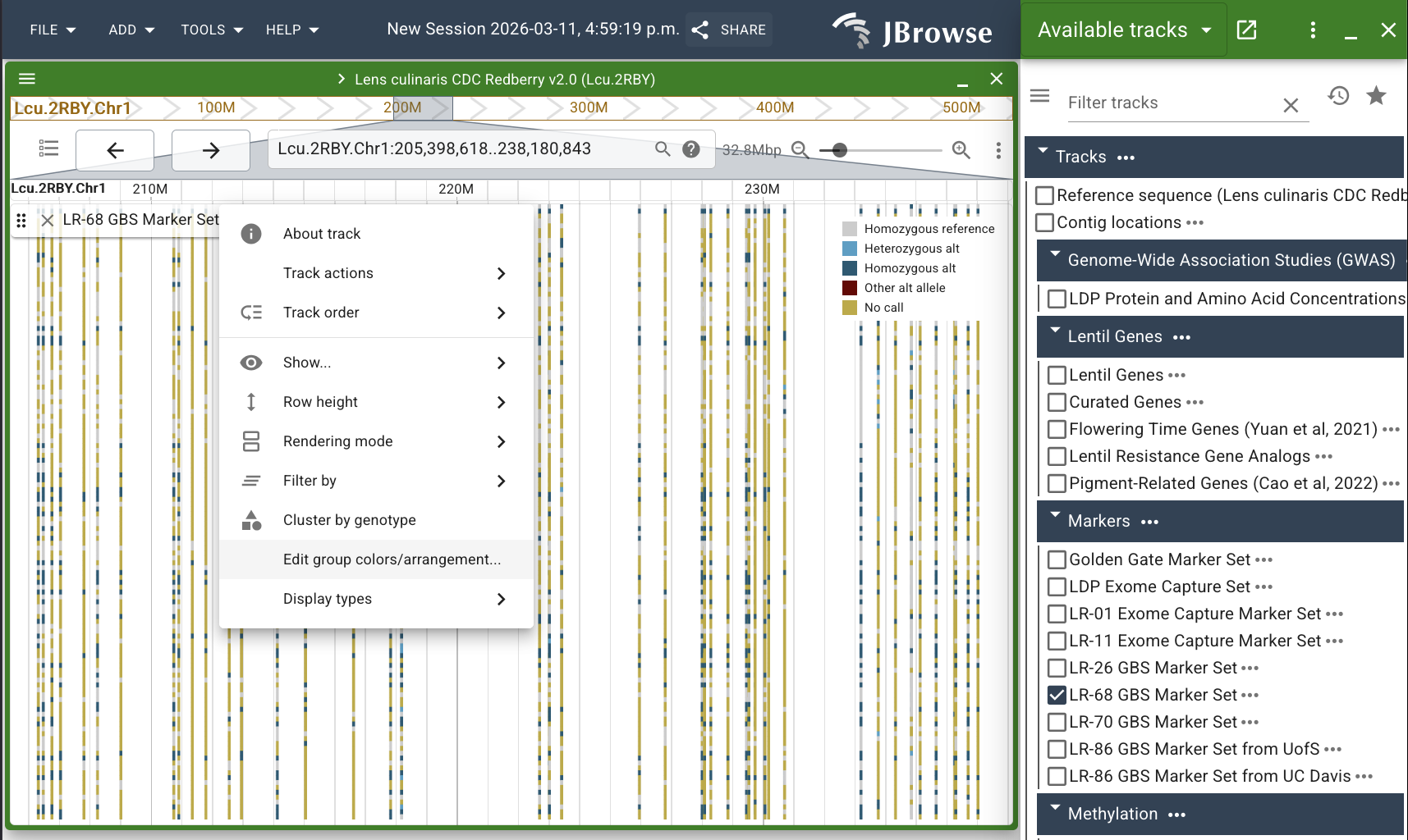
Click next to the track name (the vertical ellipsis) and select "Edit group colors/arrangement..." from the list.
A pop-up with a table will appear, containing the sample names for the LR-68 GBS marker set and another column for "Color". We are going to add a new row to this table which contains the values of our white-purple flower trait for each sample.
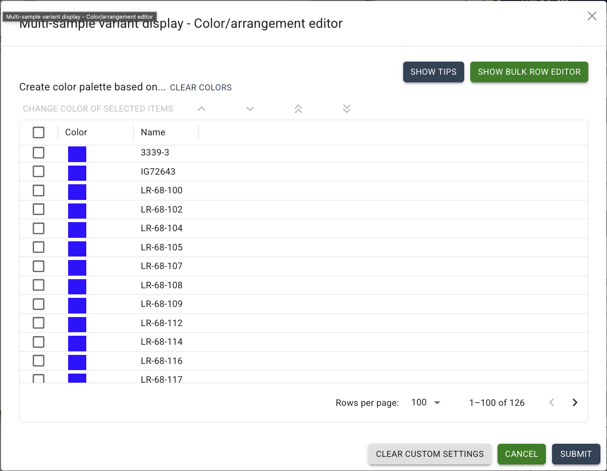
Click on "SHOW BULK ROW EDITOR" in the top right, and a textbox will appear.
Open your downloaded text file for our trait in a text editor or Microsoft Excel. If you are using Excel, check the file for automatic renaming that often occurs when Excel thinks a name is actually a date. In our file, this is likely to happen to our first sample, the maternal parent 3339-3.
When creating your own trait file, ensure that all sample names match exactly with the sample names used in the table in JBrowse. If using a column header for your phenotypic data, the first column must be "name" with all lowercase. The column(s) for your trait(s) can be named however you like. Copy and paste the two columns of data (name and White-Purple Flower Colour (scale)) into the textbox in JBrowse.
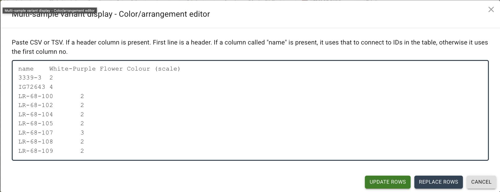
Click "UPDATE ROWS". You should now be returned to the table of samples, and a new column has been added for your trait. (Troubleshooting tip: If you don't see an added column to the table, check your sample names and try it again. It is a little finicky and doesn't provide much feedback if something is wrong in your file.)
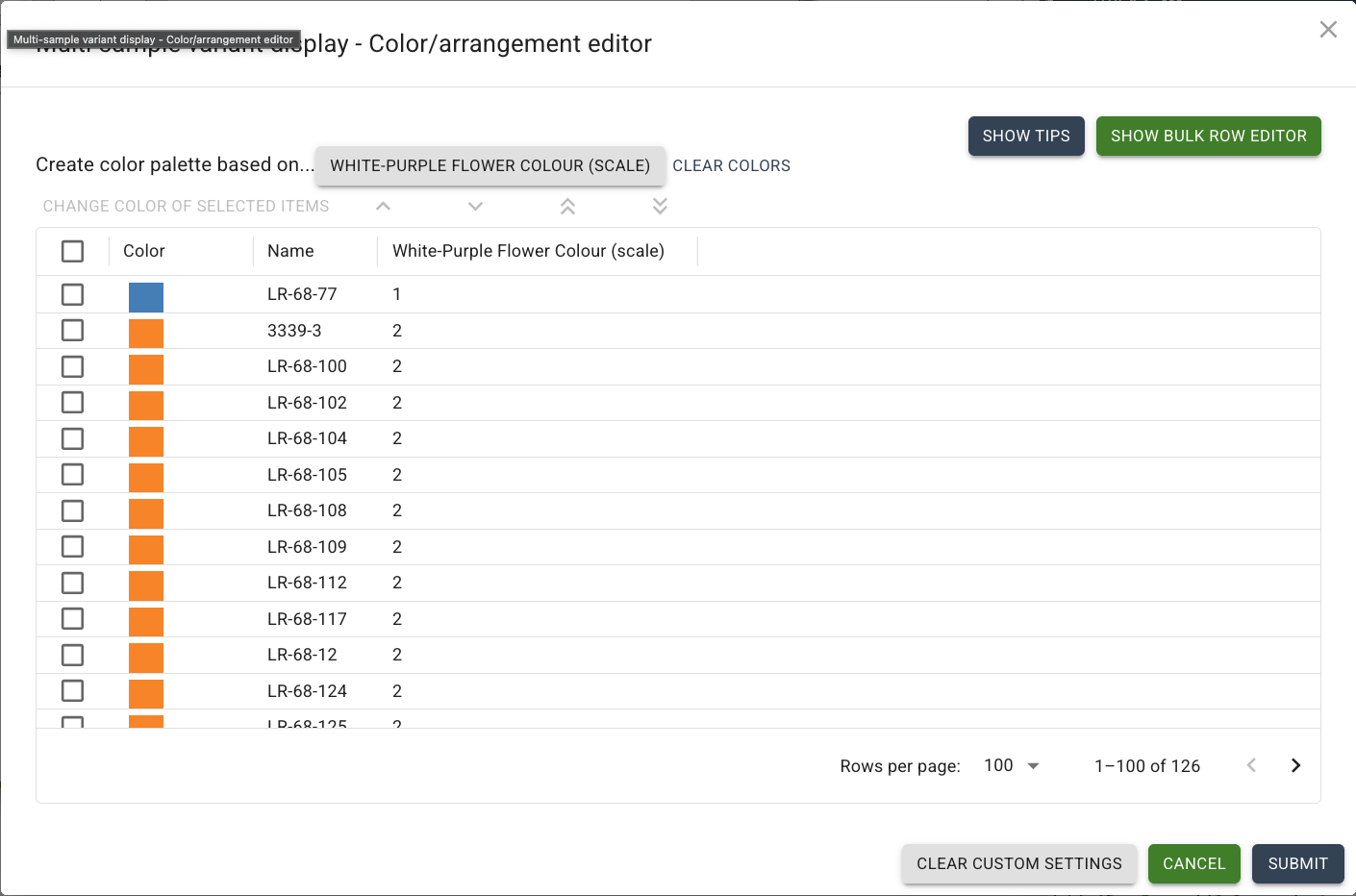
To automatically colour the samples based on your trait values, click on the grey button with your trait name, in this case, "WHITE-PURPLE FLOWER COLOUR". You can also sort your trait values, so that the samples are grouped by the value of the trait. Finally, click "SUBMIT" to see the samples coloured and sorted accordingly on the track.
2. Viewing your own GWAS results as a track
For this case study, suppose you have performed a GWAS analysis and want to visualize your results in JBrowse. Typically, GWAS results are displayed as a Manhattan plot, where SNPs are displayed as dots along the length of the genome. SNPs which are more significantly associated to the trait of interest will appear higher on the plot than less significantly associated SNPs. You can add your own track to the JBrowse in order to take a look at your GWAS results before refining the dataset, to share the preliminary results with colleagues, or to save an image for a publication/presentation.
To add your own track to JBrowse, you will need to have your data in a supported file format. For GWAS results, the output typically looks similar to BED format: a tab-delimited text file that contains the chromosome and position of each SNP and it will need to contain a column with a score attribute, which is the p-value of the SNP that has been -log10(p) transformed. Note that typically a BED file contains a column for the start position and a column for the end position of a feature. For SNPs, the start and end position will be the same, so we can either modify our file to duplicate the start position column, or we can index the file using software called tabix and ask tabix to pull both start and end coordinates from the position column. To add a GWAS track, your file is required to be tabix-indexed regardless, so I suggest you take the second approach. To do this, you will need to download and install htslib. Then, navigate to your file on the command line and run the following commands:
bgzip -k [your GWAS file]
tabix -s 1 -b 2 -e 2 --csi [your GWAS file].gz
Tabix will create an index file in addition to your bgzipped file. The -b and -e options are asking tabix to pull the start and end coordinates of each SNP from column 2. The --csi option is needed to tell tabix to create a CSI index rather than TBI (which is default). This is due to the length of Lens chromosomes, so always add -csi when indexing anything Lens!
For this tutorial, we will use a dataset of significant SNPs from a GWAS analysis on days to flower from this publication: Focusing the GWAS Lens on days to flower using latent variable phenotypes derived from global multienvironment trials.
Click here to access Supplemental Table 1 on Github.
Take a look at the file in its current format - do you think it is BED-compliant? What modifications do you think we will need to make to the file in order to add it as a track to JBrowse?
Click here to reveal modifications needed
To be considered a BED file, the first column must be the chromosome name and the second column must be the position on the chromosome. Not only are the chromosomes listed in column 2, but they are also missing the prefix that JBrowse expects to refer to the genome assembly. So to prepare this file, we would need to move chromosome and position (columns 2 + 3) to column 1 and 2 respectively, and then add the prefix "Lcu.2RBY.Chr" to the chromosome number in column 1.
The final processed file and its index can be downloaded here:
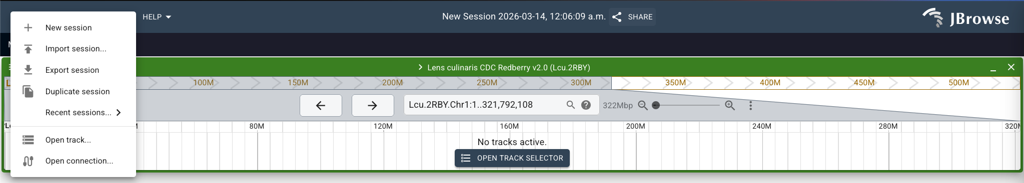
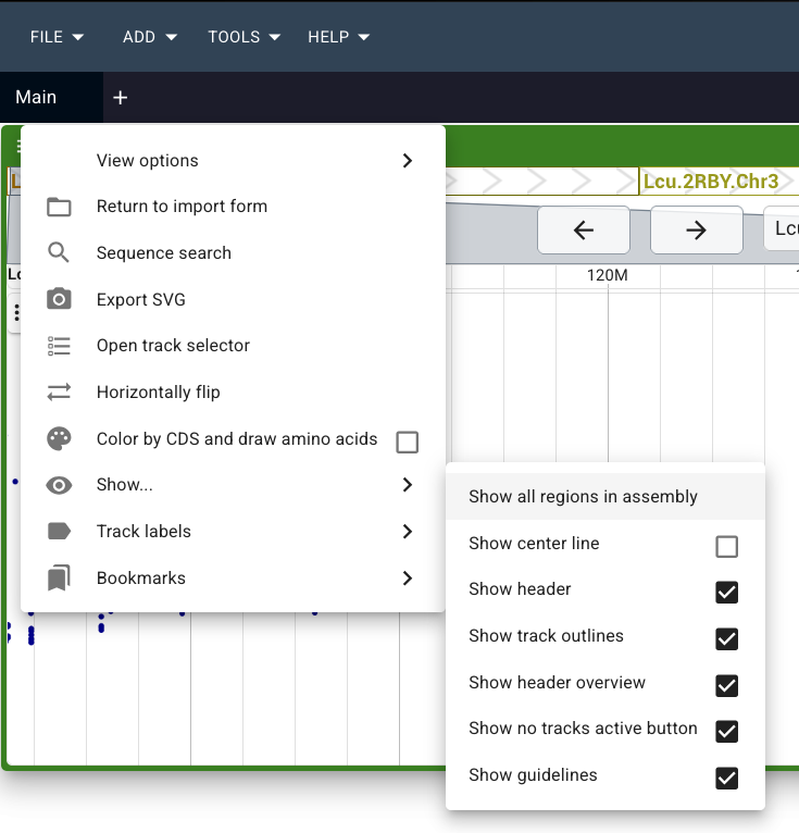
Now that we have our files, navigate to the Lcu.2RBY assembly in JBrowse and choose "Show All Regions in Assembly". Go to "File" > "Open track.." and you'll see an upload form where the track listing usually is.
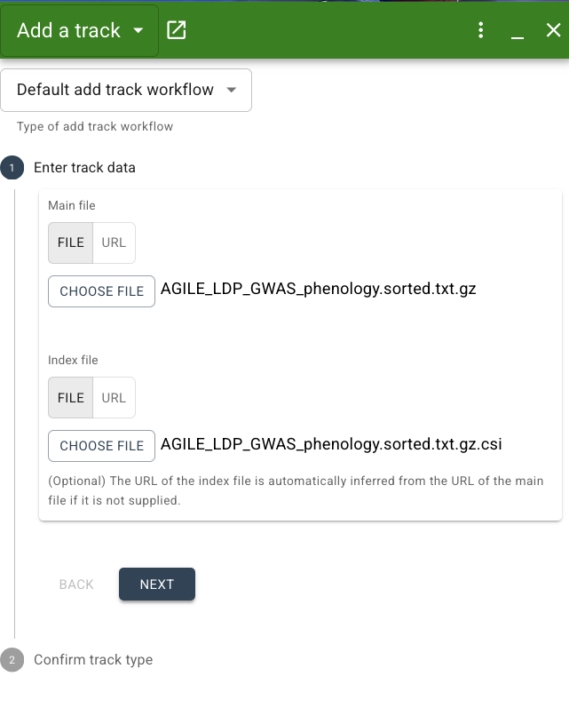
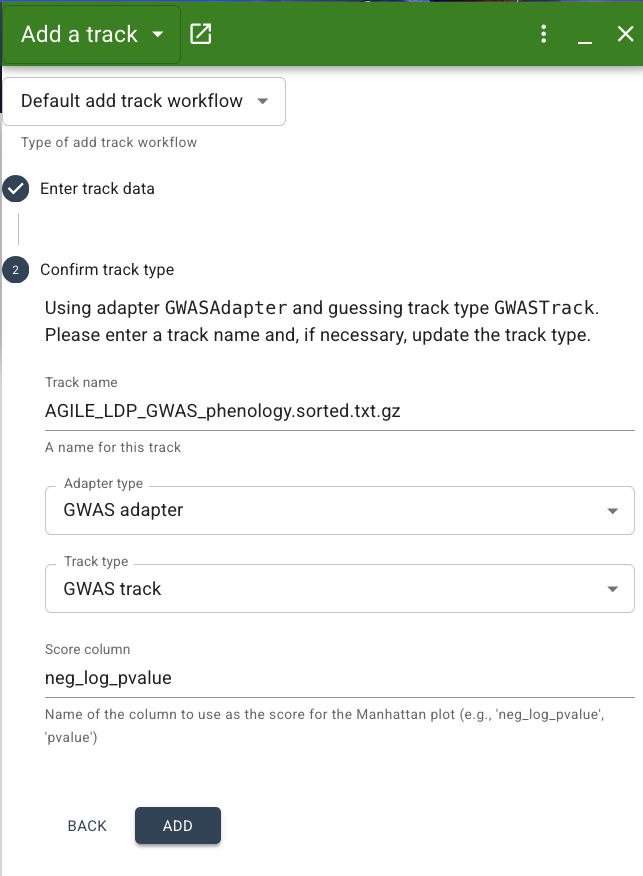
Stick with the "Default add track workflow" option. To enter track data, choose "FILE" (default is "URL") and upload the bgzipped file: "AGILE_LDP_GWAS_phenology.sorted.txt.gz". Then under index file, choose the index file "AGILE_LDP_GWAS_phenology.sorted.txt.gz.csi". Click "Next".
Next step is to confirm the track type. By default, JBrowse will make its best guess at the adapter and track type based on the file format, but you can also specify the track type if you know it. For our dataset, the correct adapter type is "GWAS adapter" and track type is "GWAS track". While a BED adapter and Feature track would both technically work for our data, we want to specify the GWAS adapter specifically since this will ensure our data is presented as a Manhattan plot. If JBrowse does not automatically select this for you, choose it from the dropdown menu. You can also specify a track name here if you'd like. Lastly, we have to set the "Score column" to the name of the column containing the negative log of the p value of our SNPs association with the days to flower trait. In our file, this column is called: -log10(p). Make sure you match this column name exactly.
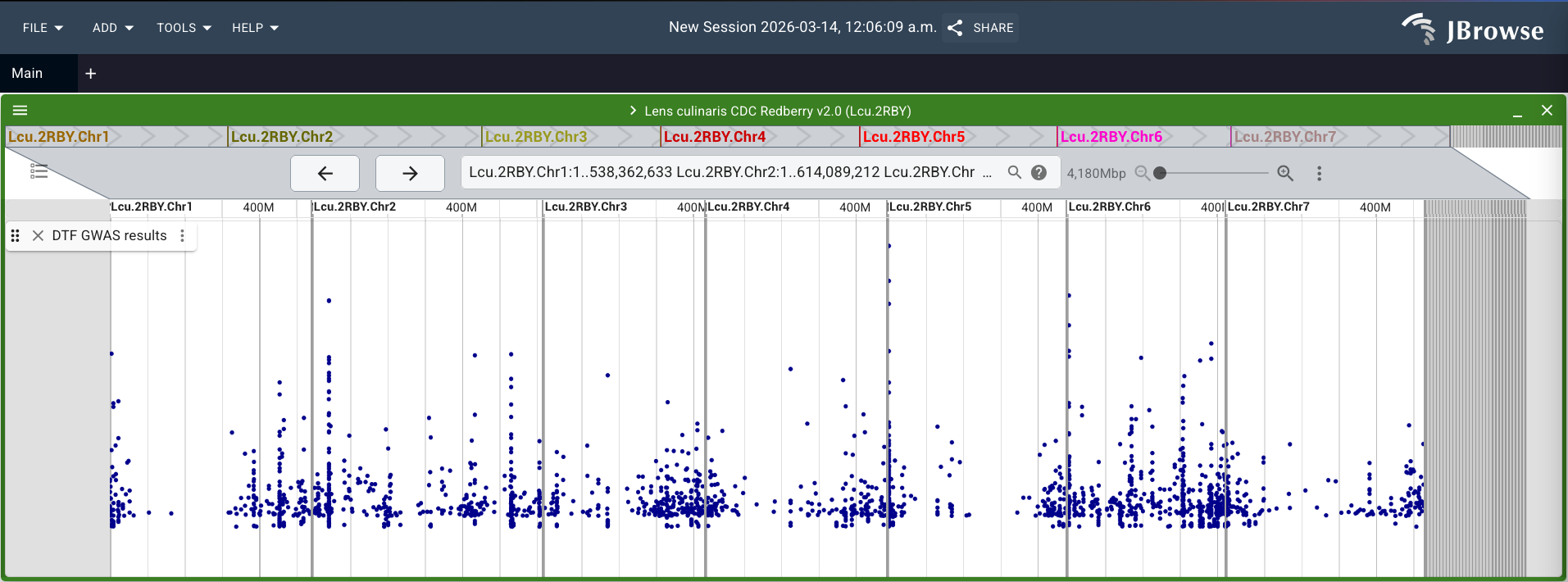
Click "Add", and your track should now appear as a Manhattan plot! NOTE: Since this dataset is already filtered for significant SNPs, that is why we see empty space below the plot. With a raw dataset, we'd expect to see a lot of dots at the bottom of the track representing the many SNPs that are not significantly associated with the trait.
TIP: If you forgot to click on "Show all regions in assembly" before adding your track and you only see a single chromosome, you can change the view after the fact by going to the 3 horizontal lines in the top left of the green bar of your view. Click on "Show..." and then select "Show all regions in assembly".
3. Demonstrating synteny between Lens species
Coming soon!